Node Expressions - Documentation

Node Expressions allows you to build the nodes of a node tree simply by typing a mathematical expression - rather than having to put together node nodes 'by hand'. This can save considerable time by avoiding the work of adding and linking multiple nodes manually and greatly reduces the risk of manual errors. The expression can be easily edited and the changes immediately re-applied to the node tree.

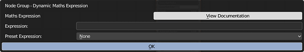
Additional documentation is avilable by clicking the View Documentation button on the above operator panel.

Basic Operators and Input Variables

At its very simplest, the expression consists of a number of input variables combined using mathematical operators - with '+' for addition, '-' for subtraction, '*' for multiplication and '/' for division, as well as '**' to indicate "raised to the power of" (eg, 'x**2' for x-squared).

The input variables can be virtually any name made up of upper and lower case letters and numbers (although it must start with a letter, rather than number). So, for example, 'x', 'y', 'z', 'Angle', 'Scale', 'SomeValue', 'Whatever', 'You', 'Want' are all valid variables. . Basic

Clicking 'OK' will validate the entered expression and automatically build the nodes for you to produce that operation, adding all the inputs you specify. For example, to add three values together you could enter the expression as :

val1 + val2 + val3

This will produce a node group with inputs of 'val1', 'val2', 'val3' containing the nodes to add all three inputs together.

Any combination of the operations can be included - and any number of inputs can be specified (variables in the expression with the same name will be automatically linked to the same input).

Additional Operators

In addition to the above mathematical operations, you can also use the following 'comparitor' operators to compare one value with another. In the case of comparisons, a result of zero indicates False, while 1.0 indicates True (ie, the same as the 'Greater Than' and 'Less Than' nodes) :

> Greater Than

< Less Than

>= Greater Than or Equal (ie, Not Less Than)

<= Less Than or Equal (ie, Not Greater Than)

== Equal To (ie, Not Greater Than or Less Than)

Operator Sequence and Brackets

Operations are applied in standard mathematical order - ie, the expression "5 + 3 * 6" would be calculated as "3 times 6, add 5" (the multiply being applied before the addition. For the above operators (+, -, *, /, **, >, <, >=, <=, ==), power ('**') is applied first, followed by multiplication and division (*, /), followed by addition and subtraction (+, -), followed by the comparator operators (>, <, >=, <=, ==).

In order to override this precedence, you can add brackets to the expression. For example, to apply the addition first in the above example, you could simply write "(5 + 3) * 6".

Named output

Any expression can be prefixed with 'XXX=' to name the output generated for that expression (where 'XXX' can be replaced with the output name). For example, the expression "Dist = (x**2 + y**2 + z**2)**0.5" will create an output socket named 'Dist' that produces an output calculated from the inputs x, y, z.

Note that you can add multiple outputs to the node group by simply listing multiple named expressions, separated by commas. For example, "Dist = (x**2 + y**2 + z**2)**0.5, Sum = x+y+z".

Mathematical Functions

In addition to the above operators you can also use various mathematical functions such as Sine, Cosine, etc. For example, you could create a simple adjustable 'wave' output using the Sine function as "Wave = sin(Input * Frequency) * Amplitude".

The following functions are available :

sin(x)

Calculate the Sine of an angle (in radians)

cos(x)

Calculate the Cosine of an angle (in radians)

tan(x)

Calculate the Tangent of an angle (in radians)

asin(x)

Inverse Sine

acos(x)

Inverse Cosine

atan(x)

Inverse Tangent (convert gradient to angle)

atan2(x,y)

Alternative Arctangent accepting two arguments (components of gradient to angle)

abs(x)

The magnitude of the value (ie, ignore the sign if negative)

round(x)

Round to the nearest whole number

max(x,y)

Determine the largest of the provided values (can list any number of input values - eg, 'max(a,b,c,d,e,....)'

min(x,y)

Determine the smallest of the provided values (can list any number of input values - eg, 'min(a,b,c,d,e,....)'

mod(x,y)

Return the Modulo (the remainder after dividing x by y) (symetrical for negative values)

mmod(x,y)

Return the Modulo (the remainder after dividing x by y) (mathematically correct modulo function)

log(x,y)

Return the Logarithm

not(a)

Invert the logical value ('True' becomes 'False', 'False' becomes 'True')

and(a,b)

Logically combine multiple values with the 'and' operator (ie, only produce 'True' if all inputs are 'True')

or(a,b)

Logically combine multiple values with the 'or' operator (ie, produce 'True' if any input is 'True')

xor(a,b)

Logical 'exclusive-or' operation

clamp(a)

Clamp the value to be within the range 0.0 to 1.0

clip(a)

Same as 'clamp'

fract(a)

Return the fractional part of a number (eg, 'fract(5.678)' would return '0.678')

floor(a)

Round down to the next lowest whole number

ceil(a)

Round up to the next highest whole number

Vectors

The individual channels of a vector can be accessed by adding a suffix to indicate the element (or channel) of the vector in square brackets ('[' and ']'). This can be either by using a numeric suffix, starting from zero; so, for example, "Vector[0]" for the first element of Vector, "Vector[1]" for the second element, "Vector[2]" for the third element. For convenience thee numeric index can be replaced with either 'x', 'y', and 'z' for the XYZ channels of a vector or 'r', 'g', 'b' for the red, green, blue channels of a Color.

Furthermore, when specifying the name of the an output to the node group you can suffix with '[]' (open and close bracket) to indicate that the output is a vector and then use the 'combine(....)' function to combine multiple elements into a new vector.

For example, you could create a node to generate a grid of coordinates using :

Output[] = combine(mod(Input[x], 0.2) / 0.2, mod(Input[y], 0.2) / 0.2, mod(Input[z], 0.2) / 0.2)

Other functions are available to manipulate vectors :

vadd(v,w)

Add two vectors together

vsub(v,w)

Subtract one vector from the other

vmult(v,w)

Multiply components of two vectors to produce new vector (v[x]*w[x], v[y]*w[y], v[z]*w[z])

vdiv(v,w)

Divide components of two vectors to produce new vector (v[x]/w[x], v[y]/w[y], v[z]/w[z])

vdot(v,w)

Return the dot-product of the two input vectors

vcross(v,w)

Return the cross-product of the two input vectors

vnorm(v)

Scale a vector so that it has length of 1.0

Defaults

When using a variable in an expression it will be added with an initial value of 0.0 unless you specify otherwise. You can specify a different default value by specifying it within '{' and '}' brackets after the variable. eg, to set the default for input Scale to '4' you can use :

ScaledX = x / Scale{4}

Special Inputs

Various inputs can be accessed via special named variables for convenience. For example, to access the Generated input coordinates of the Texture Coordinates node you can simply use 'Input.Generated' in your expression, or 'Input.Object' for Object coordinates. This can be combined with Vector subscript suffix and so, for example, to access the 'x' coordinate of the Generated coordinates you can simply use 'Input.Generated[x]' in your expression.

In addition, certain mathematical constants are available to use in your expression by including a quoted string - for example "pi" for the value of Pi (approximately 3.141).

To demonstrate this in action, consider the following expressions :

Output = sin(Input.Object[x] * 2 * "pi" * Frequency{1}) * Amplitude{1} > Input.Object[y]

In the above expression we're using Input.Object for Object coordinates and splitting out the 'x' and 'y' coordinates using the vector notation. The 'x' coordinate is used in a Sine function, multiplied by 2 * pi * Frequency and the result multiplied by an Amplitude input. Both of the input variables (Frequency and Amplitude) have defaults of 1.0. This produces the following node group :

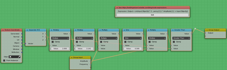
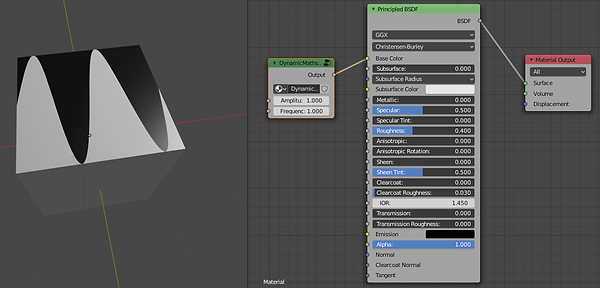
This produces the following result :

Other Functions

Various functions are available so that you can use Texture nodes in your expression :

Musgrave

musgrave(vector,scale,det,dim,lac,off,gain)

The musgrave function adds a Musgrave Texture node to your expression. The first argument (vector) specifies the input vector to the group, while the others set the various parameters for the texture (scale, detail, dimension, lacunarity, offset, gain - as for the actual node). Omitting the parameter arguments will leave those inputs set to the Musgrave Texture defaults

The last 5 arguments are optional and defaulted if not present.

The musgrave node includes a 'mode' setting which can be set to any of 'fBM', 'Multi-Fractal', 'Ridged Multi-Fractal', 'Hetero Multi-Fractal' and 'Hetero Terrain', with the default being 'fBM'. Adding a suffix to the 'musgrave' function name allows the 'mode' to be set :

fBM (default):

musgrave.fbm(vector,scale,....)

Multi-Fractal:

musgrave.mf(vector,scale,....)

Ridged Multi-Fractal:

musgrave.rmf(vector,scale,....)

Hetero Multi-Fractal:

musgrave.hmf(vector,scale,....)

Hetero Terrain:

musgrave.ht(vector,scale,....)

Voronoi

voronoi(vector, scale)

Similar to Musgrave, you can use a 'voronoi' function to include a Voronoi texture in your expression. The default mode for voronoi is for 'intensity' mode. Other modes can be used by including a suffix to the function name.

Cell:

voronoi.cell(vector, scale)

Crackle (Blender 2.8+):

voronoi.crackle(vector, scale)

Closest Distance Intensity (closest, 2nd closest, 3rd closest, 4th closest) (Blender 2.8+)

voronoi.distance1(vector, scale)

voronoi.distance2(vector, scale)
voronoi.distance3(vector, scale)
voronoi.distance4(vector, scale)

Point Density

point(vector, mode, object, [particlenum,] radius, resolution, vertexweightattr, options...)

'mode' be either PARTICLE or VERTEX to indicate the source from a particle system or the mesh vertices.

'object' is a quoted string (eg, '"Cube"') indicating the object for the source of the particle system or vertices

'particlenum' is the index of the particle system to use (for PARTICLE mode only)

'radius', 'resolution', vertexweightattr' are optional (vertexweightattr is only used for VERTEX WEIGHT mode)

'options' is a list of additional options to set up the point density (can be specified in any sequence - up to one from each set):

OBJECT/WORLD set the Space

LINEAR/CLOSEST/CUBIC set the Interpolation

COLOR/WEIGHT/NORMAL set the Color(Vertex mode only)

VELOCITY/SPEED/AGE set the Color (Particle mode only)

point.density(vector, .....) As above but using 'Density' output

Example : point.density(Input, PARTICLE, "Cube", 1, 0.45, 150, WORLD, CLOSEST, AGE)

Color Ramp

colorramp(value, [options,] valuel1, color1, ...)

List any number of 'value', 'color' pairs to set each point in the color ramp. Note that the 'color' can be specified either as a value (for greyscale) or as a vector by using the 'combine(...)' function. 'options' are optional and configure the Color Ramp from it's defaults. Valid options are:

RGB/HSV/HSL set the color mode

NEAR/FAR/CW/CCW set the hue interpolation

EASE/CARDINAL/LINEAR/B_SPLINE/CONSTANT set the interpolation

Example : colorramp(Input.Generated[x], B_SPLINE, RGB, 0, 0, 0.5, combine(0.25, 0.5, 0.75), 1.0, combine(1.0, 1.0, 1.0))

Inputs

inputs(var1, ....)

Define the 'input' variables for this group (or sub-group). This can be used instead of prefixing 'hidden' variables with '_', by defining the list of 'external' variables to be visible on this group.

Outputs

outputs(var1, ....)

Define the 'output' variables for this group (or sub-group). This can be used instead of prefixing 'hidden' variables with '_', by defining the list of 'external' variables to be visible on this group.

Note how the group node does not include a coordinate input since the expression used the 'Input.Object' special variable to automatically connect to a Texture Coordinate node.

The following special input variable names are supported :

Texture Coordinate

Input.Generated
Input.Normal
Input.UV
Input.Object
Input.Camera
Input.Window
Input.Reflection

Geometry

Geom.Position
Geom.Normal
Geom.TrueNormal
Geom.Tangent
Geom.Incoming
Geom.Parametric
Geom.Backfacing
Geom.Pointiness

Object Info

Object.Index
Object.Material
Object.Random
Object.Location

Particle Info
Particle.Index
Particle.Age
Particle.Lifetime
Particle.Location
Particle.Size
Particle.Velocity
Particle.AngularVelocity
Particle.Random

Text Blocks

Simple expressions can be entered directly into the Expression text field on the Node Expressions popup window. However, for more complicated expressions it is more versatile to enter your expression into a text block using the Text Editor window. This allows the expression to be laid out over mulitple lines and can include additional spacing and comments to aid readability. When using a text block you tell Node Expressions the text block to use for the expression using the 'TEXT:' prefix - so entering the expression as 'TEXT:mytextblock' will build the expression using the text block named 'mytextblock'.

See Making the Most of Node Expressions tutorial for additional detail.

User Defined Functions

In addition to the functions already available (Sine, Cosine, Musgrave, etc.), you can also define additional functions to use in your own expressions that can be used in the same way. This provides a method of encapsulating functionality within a sub-group that can be conveniently used multiple times which can greatly improve the readability and maintainability of your expressions.

A function allow you to define an expression with a single output and give it a name that you can reference elsewhere to include that expression using different inputs. For example, you could create a function to, say, multiply two vectors together and then use that function in your own expressions - or to perform some calcualtion that you want to repeat or reuse.

To define a function you start with a 'function:start(...)' line to define where the function begins, give it a name, and define its inputs - eg, 'function:start(myfunction, v1, v2, v3)'

The following line(s) define the body of the function (what it actually does) - eg, 'Result = v1 + v2 * v3'

The function is completed with a 'function:end(...)' line to indicate where it ends - eg, 'function:end(myfunction)'

The function is used by prefixing the name with 'fn:' - eg, 'fn:myfunction(x,y,z)'

As an example, consider the following expression text block to define and use a function to calculate the 'absolute' value of each of the elements of a vector :

function:start(vabs, Vector)

Result[] = combine(abs(Vector[x]), abs(Vector[y]), abs(Vector[z]))

function:end(vabs)

You can then use the function in the subsequent expression as follows :

fn:vabs(v)

The function can then be used in your own expressions.

Sub-groups

A 'function' can be used to define a reusable expression with any number of inputs but only a single output - so it can be used inline in your expression to produce a single output. If you require a sub-node with multiple outputs you can use similar syntax to define a 'group'; a 'group' can have any number of inputs as well as any number of outputs - each of which can be accessed individually. The only practical difference between a 'function' and a 'group' is how you "invoke" it.

To define the start of the group you use a 'group:start(...)' line to start the group - specifying the name and inputs to the group, similar to a function definition.

The body of the function can then be defined - this is effectively the contents of the group, defining the outputs for the group.

The end of the group is indicated using a 'group:end(...)' line.

Once created, you can include the group in your own expression using 'group:add(...)', specifying the group name, the 'instance' name (what this sub-group will be referred to in your expression) and the inputs to the group.

To use the output of the group in your expression you can use the 'group:<instancename>[output]' syntax.

The 'Mandelbulb' preset demonstrates the use of groups by defining a group for one iteration of the mandelbulb calculation and adding multiple groups to the expression, chaining each one to the subsequent group :

# Mandelbulb : Generate a Mandelbulb (3d-mandelbrot)

#Define the group for one 'iteration' of the Mandelbulb calculation
group:start(mandelbulbiteration, N, iBlown, Limit, iOffset[], iVector[])

#Split the input vector into x,y,z
_x = iVector[x]
_y = iVector[y]
_z = iVector[z]

#Calculate the coordinates
_r = (_x*_x + _y*_y + _z*_z)**0.5
_theta = atan2((_x*_x+_y*_y)**0.5,_z)
_phi = atan2(_y,_x)

_rn = _r ** N

_newx = _rn * sin(_theta*N) * cos(_phi*N)
_newy = _rn * sin(_theta*N) * sin(_phi*N)
_newz = _rn * cos(_theta*N)

#New distance from centre
_newR = (_newx*_newx + _newy*_newy + _newz*_newz)**0.5

#Determine whether our new point lies outside the sphere
oBlown = or(iBlown, _newR> Limit)

oVector[] = vadd(combine(_newx, _newy, _newz), iOffset[])
Intensity = _r - _newR

#End the group - the name should match the 'start'
group:end(mandelbulbiteration)

#-----------------------------------------------------------------------------------------

#Add a group node named 'iteration1', setting the inputs to the group input values
group:add(mandelbulbiteration,iteration1,N{8},0,Limit{2},Input[], Input[])

#Add second group node named iteration2 and linked to the first
group:add(mandelbulbiteration,iteration2,N,group:iteration1[oBlown],Limit,Input[], group:iteration1[oVector])

#Add some more iterations
group:add(mandelbulbiteration,iteration3,N,group:iteration2[oBlown],Limit,Input[], group:iteration2[oVector])
group:add(mandelbulbiteration,iteration4,N,group:iteration3[oBlown],Limit,Input[], group:iteration3[oVector])
group:add(mandelbulbiteration,iteration5,N,group:iteration4[oBlown],Limit,Input[], group:iteration4[oVector])
group:add(mandelbulbiteration,iteration6,N,group:iteration5[oBlown],Limit,Input[], group:iteration5[oVector])
group:add(mandelbulbiteration,iteration7,N,group:iteration6[oBlown],Limit,Input[], group:iteration6[oVector])
group:add(mandelbulbiteration,iteration8,N,group:iteration7[oBlown],Limit,Input[], group:iteration7[oVector])
group:add(mandelbulbiteration,iteration9,N,group:iteration8[oBlown],Limit,Input[], group:iteration8[oVector])
group:add(mandelbulbiteration,iteration10,N,group:iteration9[oBlown],Limit,Input[], group:iteration9[oVector])

#Define the outputs
Inside = not(group:iteration10[oBlown])
Intensity = group:iteration10[Intensity]

Presets

The add-on includes various 'preset' expressions that can be chosen from the Preset Expression drop-down when adding a new expression. These are provided as potentially useful expressions as-is, as well as providing various examples to either use in your own projects or to use as the basis of your own expressions. By enabling the 'Create as Text Block' checkbox, the add-on will create a new text block containing the text of the expression that can be viewed and edited as required.

Imports/Includes

In order to provide a convenient method of including functions and groups in your own expressions without having to define a copy of the function/group expression in each of your own expressions, you can use the 'import(...)' function to import an expression or function/group definition from another text block.

For example, if a textblock exists named 'myfunctions' with definitions of all the functions you want to use in your own expression (using the syntax described above) then you can include them in your own expression with :

include "TEXT:myfunctions"

For convenience (and familiarity with other language syntax) you can replace the keyword 'include' with 'import' for the same result. eg,

import "TEXT:myfunctions"